Mapping Early American Elections

QGIS Tutorial

Brandan P. Buck April 30, 2019

Enjoyed looking at the maps featured on the Mapping Early American Elections (MEAE) site? Wish you could utilize the MEAE dataset to make your own maps, but are not sure how to get started? You’re in luck! The following tutorial will teach you how to combine MEAE data with historical geospatial data in QGIS to create basic choropleth maps (maps which show geographic regions colored or shaded according to some variable).

While we are going to demonstrate how to make maps for Maryland’s First Congressional election, these steps can easily be replicated to create maps for different Congressional elections and for different states. By the end of this tutorial, you will have learned how to make a map similar the MEAE map for Maryland’s 1st Congress.

Tutorial Overview and Goals

In this tutorial, we will be using QGIS, an open-source desktop geographic information system (GIS) application used for viewing, editing, and analyzing geospatial data. We will use QGIS to manipulate MEAE elections data for Maryland’s First US Congressional election and create two visualizations in the form of choropleth maps. By the end of this tutorial you will have learned how to:

Retrieve MEAE elections data for a selected state.
Obtain historical spatial data for a selected state.
Merge and manipulate the MEAE elections data with the geospatial data for further analysis.
Visualize this data geographically by creating choropleth maps of (1) party percentages and (2) an individual candidate’s votes.

Getting Started

This tutorial will assume that you already have set up QGIS, and have a basic knowledge of how the tool works. (If not, QGIS can be downloaded here. An introduction to QGIS can be found here.)

Create a new QGIS project.
1. Launch QGIS.
2. Project -> New
3. Name your new project.
4. Save Project.

About the Data

In this tutorial, we will be analyzing and visualizing MEAE data which represents the election of six U.S. Congressmen from Maryland who made up the state’s delegation to the inaugural meeting the U.S. House of Representatives in 1789.

In early America, and especially for the first Congress, U.S. Congressional elections were quite experimental. Each state set its own date for elections, and devised their own voting methods and procedures. In Maryland, elections for the First Congress were held over the course of a five-day period in January of 1789. Maryland used a combination of an at-large and district voting system for the first Congress. The state was divided into six residential districts. When voters went to the polls, they cast a vote for six different candidates—each one having to reside in a different district. At the end of the election, the votes were tallied state-wide. The six candidates with the most total votes across the state were elected, regardless of their residential district. While political parties as we know them did not yet exist, the candidates had split into two competing factions known as the Federalists (in favor of Washington, Hamilton and the U.S. Constitution) and the Anti-Federalists (who opposed the ratification of the U.S. Constitution). In Maryland’s First Congressional election, all six of the winning candidates were affiliated with the Federalist faction.

The MEAE elections data we will be using in this tutorial, once downloaded, is structured as two separate .csv files (which are like spreadsheets), and it is recorded at the county level. The file congressional-parties-meae.congressional.congress01.md.county.csv (download here) has eighteen rows of data and records the number of votes and percentage of vote received by each “party” or faction in each of Maryland’s eighteen counties. The file congressional-candidates-counties-meae.congressional.congress01.md.county.csv (download here) has 324 rows of data, with each row showing the number of votes a single candidate received in one of Maryland’s eighteen counties. We will look more closely at the elections data and the variables in each file after we import the files into QGIS.

We will be joining our MEAE data to county-level historical spatial data from the Atlas of Historical County Boundaries. Maryland county shapefiles from AHCB can be downloaded from their website.

Readying Elections Data for Analysis

Importing the MEAE Data

Start by downloading the necessary elections return data. For this tutorial you will use election returns for Maryland’s first congressional elections in 1789. You will need returns for both parties and individual candidates to complete this tutorial in its entirety. The data is available from an MEAE GitHub repository. The data for party results by county is stored in this directory: you want the .csv file for Maryland’s first Congressional election. You should also download the file for individual candidate results by county from this directory, which you will use later in this tutorial.

In addition, you will need to create .csvt files for each election return .csv. QGIS will automatically reformat the data to strings and thereby prevent you from being able to format them properly. In order to use the QGIS features you will need you will need to tell QGIS how to format the data. It is imporant that you enter the following text verbatim. Creating a companion .csvt file for both the party and individual returns will allow you to complete the maps.

Download the appropriate elections data here.
Create csvt files for congressional-parties-meae.congressional.congress01.md.county.csv data set using Notepad for PC or TextEdit for Mac or similar programs.
1. Open your text editing program.
2. Write: 'String','String','String','String','Integer','Real','Integer','Real'
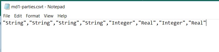
1. Save file as congressional-parties-meae.congressional.congress01.md.county.csvt (note the changed file extension) in the same folder as the corresponding .csv file.
Create a .csvt file for the congressional-candidates-counties-meae.congressional.congress01.md.county.csv data set using Notepad for PC or TextEdit program for Mac or similar programs.
1. Open another window for your text editing program.
2. Write: 'String','String','String','String','String','String','String',
  'String','String','String','String','String','String','Integer'. Note that this should on one line; there is a line break here only for display purposes.)
3. Save file as congressional-candidates-counties-meae.congressional.congress01.md.county.csvt in the same folder.
Open your QGIS project.
Add the newly downloaded .csv files to your QGIS project via “Add Layer”, “Add Delimited Text Layer.” Select the “No Geometry (attribute only table)” box.
Click ok.

Now the elections return data will function as a data layer within QGIS and appear within your Layer’s Panel on the left side of your display. The .csvt files you created will force QGIS to categorize the as it was meant to be used and will allow you to create your desired map using the “graduated” function.

Let’s take a closer look at both data objects to make sure that our data was read in correctly, and that we understand the different variables they contain. Look at the Layers Panel on the left side of your screen. You should see the two .csv files you imported. The number of observations corresponds with the number of rows of data, while the number of variables corresponds to the number of columns in the data. congressional-candidates-counties-meae.congressional.congress01.md.county.csv should have 324 observations while and congressional-parties-meae.congressional.congress01.md.county.csv should have 18 rows. Right click on a .csv in your Layers Panel and select Open Attribute Table to inspect your data.

Let’s take a closer look at the data in the parties file. This data object should contains data for the vote and percentage of the vote all parties received in this election. The first variable (column) is called meae_id. This variable contains a unique name that identifies this election in the MEAE data. You will notice that all eighteen rows have the same meae_id: meae.congressional.congress01.md.county. This tells us that all the data here is county-level data from Maryland’s First U.S. Congressional election. The variables county_ahcb and county_fips each contain a unique code for each county. Notice that each row of data represents one of Maryland’s eighteen counties. These variables will be necessary when we join the MEAE data to the spatial data.

Next, the variable districts gives information about the voting procedures in a particular election.As mentioned above, Maryland used a combination of an at-large and a district system. But to keep things simple, this election is listed as “At-Large” because voters elected six candidates that represented all voters of the state (instead of just a district or subset). Finally, the last type of variable lists the total number of votes (federalist_vote) and percentage (federalist_percentage) of the vote achieved by each party or faction. Notice that the data in the percentage columns is written as a decimal with a range of zero to one. In Maryland’s first Congressional election, only the Federalist and Anti-Federalist factions received votes. If you scroll to the right, you will see variables for other parties and factions that did not participate in this election. The data for these variables should appear as “NA.”

Now, let’s take a closer look at the data in candidates file by clicking the data object’s name in the Layers Panel.

We notice that this data object contains data for all the candidates that received votes in this election in Maryland. The first variable (column) is called election_id. Similar to the meae_id in the previous set of data, the election_id is an unique name that identifies this election. You will notice that all 324 rows have the same election_id “md.uscongress.1789”, telling us that all of this data represents the U.S. Congressional election taking place in Maryland in 1789. Again, the county_ahcb and county_fips variables used for joining this data to spatial data appear. The last four variables represent the candidate’s name, a unique ID for each candidate, the party or faction the candidate represented in this election, and the number of votes the candidate received in the county listed in that row. For example, the first eighteen rows represent the votes that candidate George Dent received in each of Maryland’s eighteen counties.

Preparing Individual Candidate Data

The map building process for individual candidates is identical to the party maps but you will need to prepare your data is a slightly different fashion to the individual candidate data structure. To ready your individual candidate choropleth map you will need to filter the results for your desired candidate.

We will need to select a variable to use to filter our data. At first, we might consider using the variable candidate, which gives the candidate’s name. However, in early America, spelling wasn’t standardized. Sometimes the first or last name of a candidate would be recorded differently in each county. Therefore, we created a variable called candidate_id which is a unique code of letters and numbers identifying each candidate in the MEAE dataset, regardless of the spelling variations of his name. If we filtered using a specific candidate’s name, we might risk not obtaining all the data for that candidate. But by filtering by the candidate_id, we make sure we get all the data for a candidate.

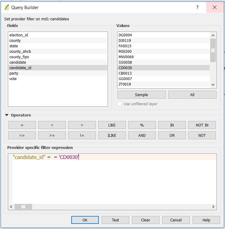
For this tutorial we will use the vote tallies for candidate Daniel Carroll. Carroll was assigned the candidate_id: CD00301. To do this you will use QGIS “filter” function and filter the candiate tallies via a SQL query. The result will allow you to append only the necessary records to your special data.

Right click on the congressional-candidates-counties-meae.congressional.congress01.md.county.csv and select filter
Select candidate_id and =
1. Click the “All” button under the “Value” window and select CD0030.
Your SQL query should look like this (see Figure 2):

candidate_id = CD0030

b.  Click ok.

Obtaining Spatial Data

In order to make this elections data geospatially valuable you will need to obtain boundary data for the state of Maryland and import that data into QGIS. You will also need to filter the data so it reflects the state’s county boundaries for 1789, the year of the election. Finally, you will export two copies of this filter data. One will be used to create a map for party data and another for election returns for an individual canidate.

Download the appropriate state shapefiles from Atlas of Historical County Boundaries. The data is located in the link “Download Shapefiles for use with GIS Programs (zip file).” Maryland boundary data can be downloaded here.
The data you will need for this tutorial is named MD_AtlasHCB. Inside you will find a folder named MD_Historical_Counties which contains the necessary file, named MD_Historical_Counties. Drag and drop the .shp file component into your QGIS Layers Panel or add it via QGIS menu Layer -> Add Layer -> Add Vector Layer.

Right click on your newly imported boundary shapefile and select “Open Attribute Table.” Let’s first look at the second through fifth variables. Compare the observation in these columns to those in either of the MEAE data objects. While the names of these new variable in md1_counties do not exactly match what we’ve seen before, the observations they contain should look familiar. The data in the new variable name matches the data for the variable county in the MEAE data; the new variable id matches the data from county_ahcb; the data in fips matches that in county_fips and so on. Having data that is common between our MEAE data and the spatial data will be key in joining the data together later on.

Next, you’ll see variables for start_date, end_date, change, and citation. When we obtained our spatial data, we stipulated that we wanted spatial data that represented Maryland counties at a specific date. The start_date and end_date show the date range for which the data provided is accurate. For example, the geographic data and boundaries provided here for Frederick County would be accurate from October 2, 1776 until January 18, 1836.

While we won’t examine every variable in md1_counties, the last variable geometry is the most important. This variable lists the exact latitudinal and longitudinal data that creates an outline of each county on a map. While it is important to inspect this data in the Source Editor and make sure that there is data listed for each county (row), it is almost impossible to tell if the data is accurate (i.e. if it will actually produce a map of Maryland) just by looking at the numbers.

Extract just the boundary data that you will need. For the 1st Congress you will require Maryland county boundaries circa January 1789. The quickest way to select the appropriate boundary will be via a SQL query.
1. First highlight the MD_Historical_Counties shapefile in your Layers Panel.
2. Open Select Features Using Expression located at the top of your QGIS tool bar and enter the following SQL query (see Figure 3):
'START_DATE' < '1789-01-01' AND 'END_DATE' > '1789-01-01'

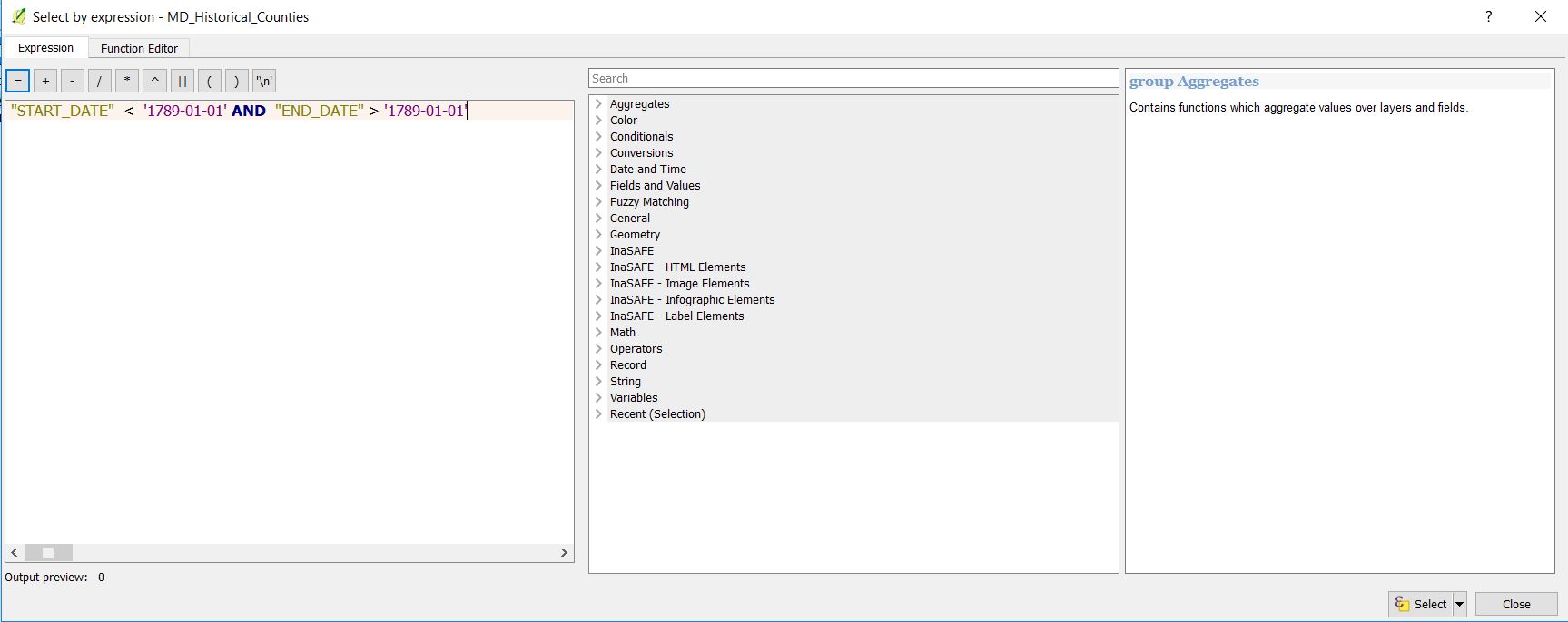
You should have 18 returns.

Note: QGIS may not properly visualize the selection; verify your success via the county shapefile attribute table.

Right click on MD_Historical_Counties.
1. Select “Save as.”
2. Select “ESRI Shapefile” from the “Format” dropdown menus.
3. Choose an appropriate file location and name.
4. Click “Save Only Selected Features.”
5. Click OK.
6. Repeat steps a through e to save an additional shapefile.
7. Import your new shapefiles into QGIS either by dragging and dropping the .shp portion of the file or via the QGIS menu Layer -> Add Layer -> Add Vector Layer.

Now you have Maryland county boundary data from 1789, the year of the 1st Maryland congressional election, and two copies depicting the boundary data.

Joining Elections Data with Geospatial Data

Joining Party Data to Geospatial Data

In order to make the desired maps you will need to join the 1st Maryland Congressional elections data to one copy of your newly created 1789 boundary data. To do so you will tell QGIS to join data from the former onto the latter using a common field. This field is referred to by slightly different naming conventions so you will need instruct QGIS as to which two fields are the same. Since you will be joining two separate fields you may want to join only that which is necessary to complete the maps.

Right click on the properties function of your 1789 Maryland county spatial data.
Select the “Joins” tab on the left side of the panel.
Select the + function on the bottom of the window.
1. Choose your party election returns .csv. from the dropdown window.
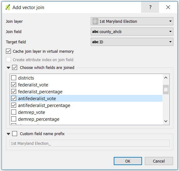
c Choose county_ahcb as “Join Field” and ID as target field.

For simplicity, you may want to join only the needed information from our election data. Under “Choose Fields Are Joined” select federalist_vote, federalist_percentage, antifederalist_vote and antifederalist_percentage (see Figure 4). Your appended sections data will appear at the end of the 1789 Maryland county spatial data spatial file

Joining Individual Candidate Data to Geospatial Data

Right click on the properties function of your 1789 Maryland county spatial data, select the Joins tab on the left side of the panel.
1. Select the + function on the bottom of the window.
2. Choose congressional-candidates-counties-meae.congressional.congress01.md.county.csv from the dropdown window.
3. Choose county_ahcb as Join Field and ID as target field, under “Choose which fields are joined” select vote (see Figure 5).
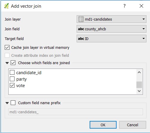
1. Your joined Carroll Daniel vote tallies will appear at the end of the 1789 Maryland county spatial data spatial file.

Now that the election information is added to your Maryland county shapefiles you can begin to build the maps using the election returns to symbolize them as desired.

Visualizing: Maps

Mapping Party Percentages

Since you joined the elections return data to your spatial data you can now use QGIS to symbolize the county polygons according to the election returns. To do so we will use QGIS’ Graduated function to create a Choropleth map.

To create a map for the Federalist Party, right click on your now exported 1789 Federalist Return shapefile, select properties.
1. Navigate to the style function and select graduated from the dropdown window select md1-parties_federalist_percentage which contains the county by county winning percentages for the Federalist Party.
2. Hit the “classify” function below the display window.
3. Select “Natural Breaks (Jenks)” for “Mode” (see Figure 6).
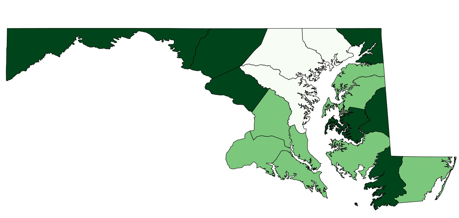
4. Choose a color scale which is aesthetically pleasing and conveys the historical information you desire for your map. For this tutorial you will use a color ramp with three values in order to convey the Federalist’s lopsided victory in the election. To do this select 3 from the “classes” drop down menu on the right side of the window. Different election results will demand a more nuanced color scale

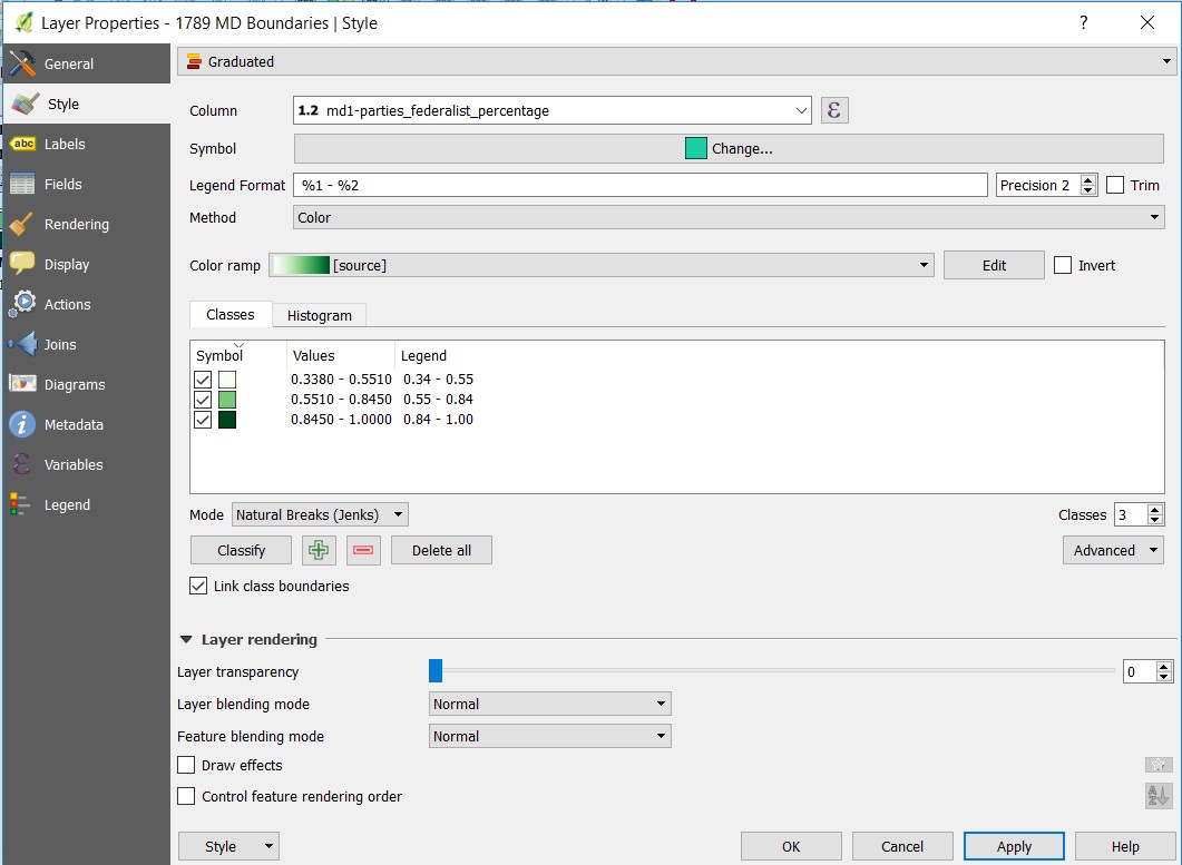
f.  Hit ok.

Export the map either via a screen grab or Project -> Save as Image. Your result should look similar to Figure 7.

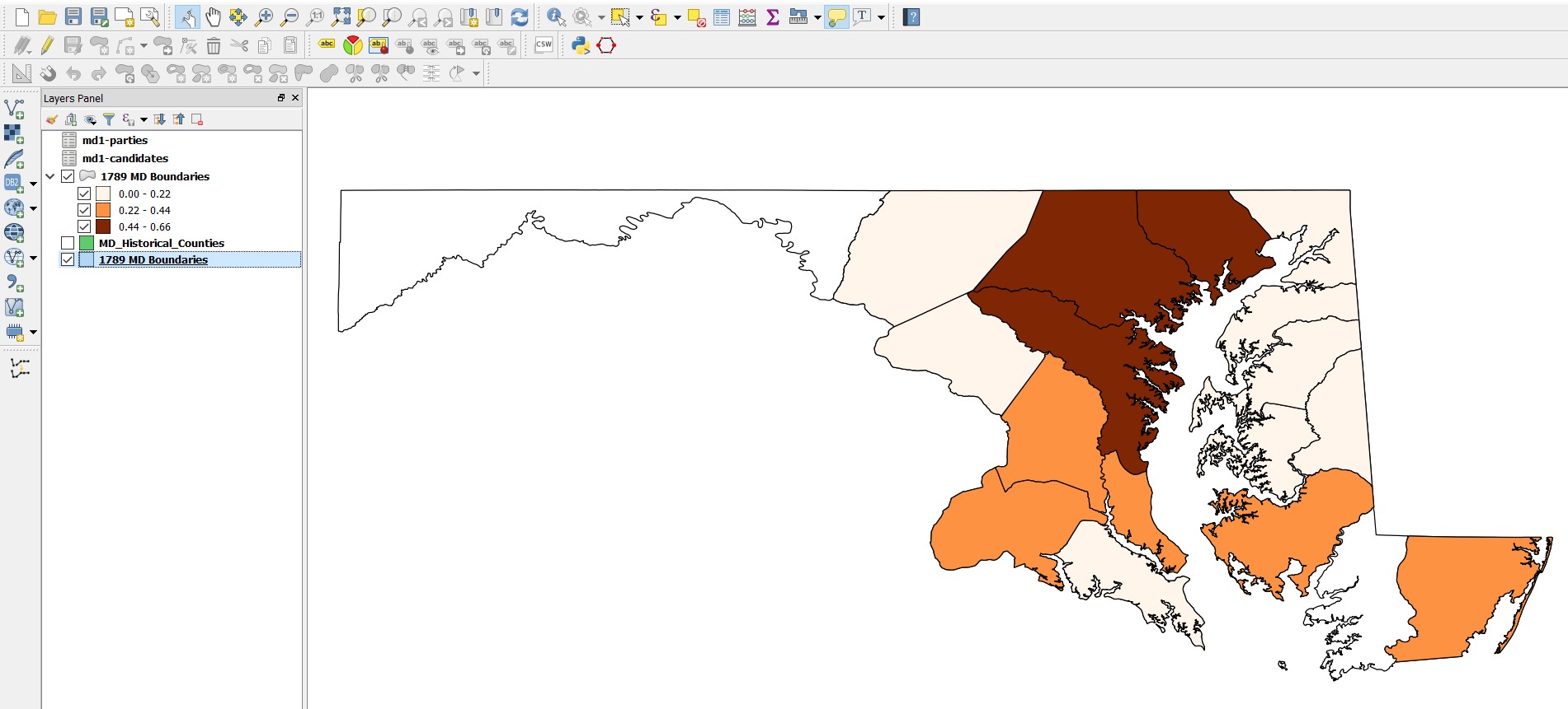
To create a map for the Antifederalist returns, repeat step one but change md1-parties_antifederalist_percentage to your input. Note, that the data has null records and therefore QGIS’ graduated function will not symbolized these counties. In order to complete your map, you will need to layer your symbolized county returns over another county shapefile shapefile, preferably one with no fill.
1. Right click on your symbolized county shapefile
2. Select “save as.”
3. Give your new boundary shapefile a name and hit ok.
4. Right click on your new boundary shapefile, select properties
5. Select “style” and highlight “simple fill.”
6. Click on the “Fill” dropdown menu, and select “transparent fill” from the box which will appear.
7. In your layers panel, drag your new, transparent fill boundary shapefile below your symbolized Antifederalist county data.
Export the map either via a screen grab or Project -> Save as Image. Your result should look similar to map seen in Figure 8.

Now you have maps for both the Federalist and Antifederalist party results for the 1st Maryland Congressional election. Both maps are properly symbolized and accurately reflect the election returns. The rest of this tutorial will instruct you on how to build similar maps for individual candidates.

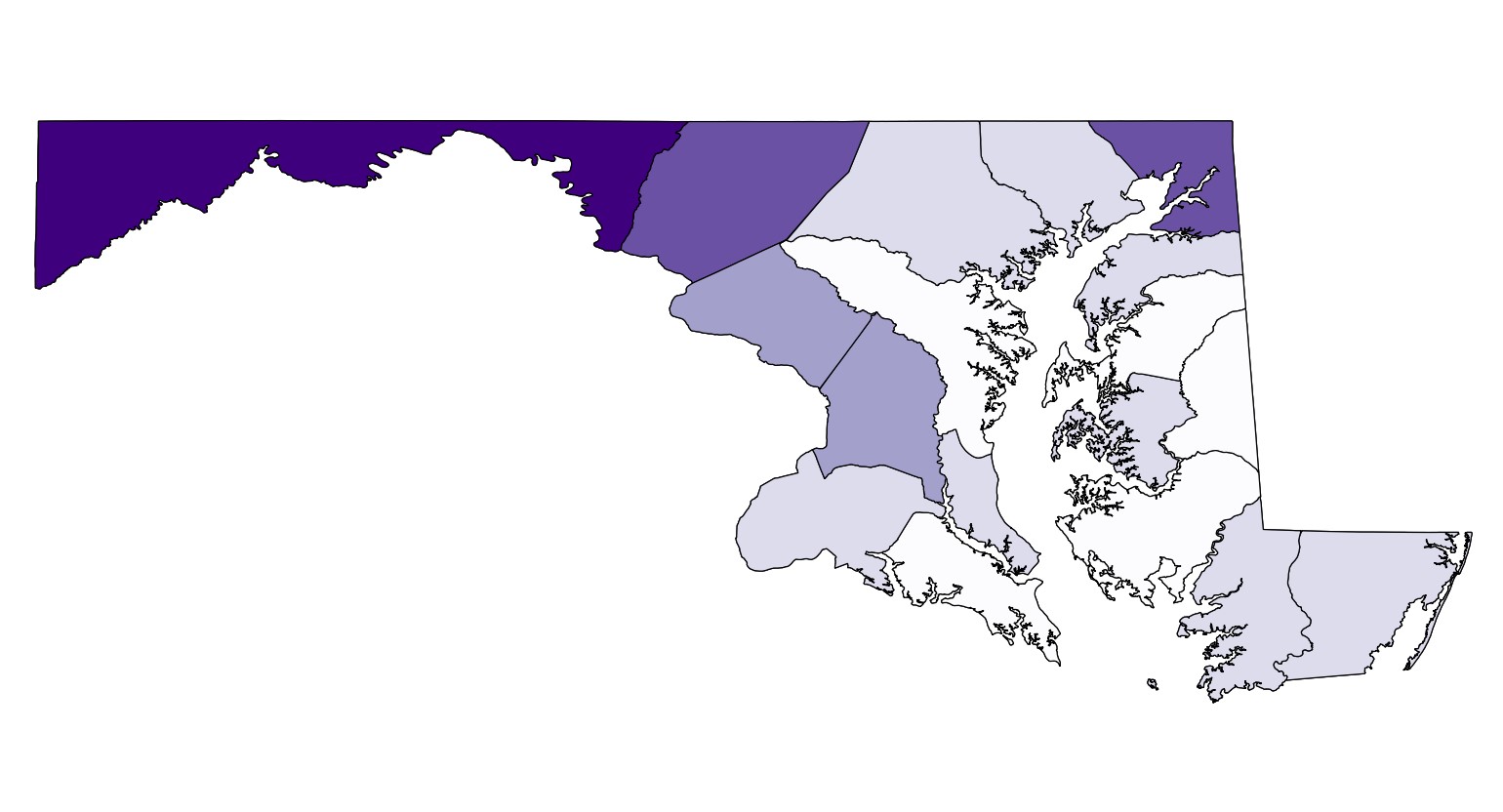
Mapping A Individual Candidate’s Votes

Mapping the individual candidates is identical to the party percentages, the only difference will be the input for QGIS’ “graduated” function.

Right click on the joined candidate boundary shapefile, select properties
Navigate to the “style” function and select “graduated” from the dropdown bat.
Select “md1-candidates_vote” which is the voting tallies for Carroll Daniel.
Select your desired color ramp, choosing a single-color ramp will allow the map to be easily read.
Hit the “classify” function below the display window.
Select “Natural Breaks (Jenks)” for Mode.
Choose a color scale which is aesthetically pleasing and conveys the historical information you desire for your map. Individual candidates may require a higher number of “classes” in order to reflect the varying votes totals per county. Five categories is an appropriate number to convey the variance in Carroll Daniel election results.
Hit ok. Your result should look similar to Figure 9.

Export the map either via a screen grab or Project -> Save as Image.
Repeat process for other candidates, beginning with the filter function, step one from Preparing Individual Candidate Data.

Conclusion

Congratulations! You have done and learned a lot in this tutorial. Just to recap, we’ve learned how to import and inspect our MEAE our data, how to obtain historical county-level spatial data, how to join the MEAE data to the spatial data, how to create party percentage maps, and how to create a map of an individual candidate’s votes.

Most importantly, this tutorial should have provided you with a basic template on how to take MEAE data and begin using geospatial analysis to analyze phenomenons such a candidate’s votes, a party’s votes, or a party’s percentage of the vote. However, this is just the beginning of the possible kinds of maps or means of inquiry you can carryout using the MEAE dataset. Using the methods outline above, you can continue to investigate by creating choropleths with other variables, and for other Congresses or other states in the MEAE dataset.